File:Partial transmittance.gif
Vai alla navigazione
Vai alla ricerca
Non sono disponibili versioni a risoluzione più elevata.
Partial_transmittance.gif (367 × 161 pixel, dimensione del file: 67 KB, tipo MIME: image/gif, ciclico, 53 frame, 4,2 s)
| Questo file e la sua pagina di descrizione (discussione · modifica) si trovano su Wikimedia Commons (?) |
Dettagli
| Descrizione |
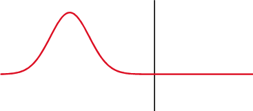
Русский: Показано классическое отражение/прохождение солитона гауссового импульса от/в более плотную среду. В реальности же, свет отражается не от поверхности, а от всех частиц тела (см. ru:КЭД). English: Illustration of partial reflection of a wave. A gaussian wave on a one-dimensional string strikes a boundary with transmission coefficient of 0.5. Half the wave is transmitted and half is reflected.
Français : Illustration de la réflection partielle d'une onde. Une onde gaussienne se déplaçant sur un ressort unidimensionnel est réfléchie/transmise au niveau d'une interface avec un coefficient de transmission de 0.5.
Español: Ilustración de una reflexión parcial de una onda. Una onda gaussiana sobre una cuerda de una dimensión choca contra un limite con un coeficiente de transmisión de 0.5. La mitad de la onda es transmitida y la otra mitad es reflejada. |
| Data | |
| Fonte | self-made with MATLAB, source code below |
| Autore | Oleg Alexandrov |
Licenza
| Io, detentore del copyright su quest'opera, la rilascio nel pubblico dominio. Questa norma si applica in tutto il mondo. In alcuni paesi questo potrebbe non essere legalmente possibile. In tal caso: Garantisco a chiunque il diritto di utilizzare quest'opera per qualsiasi scopo, senza alcuna condizione, a meno che tali condizioni siano richieste dalla legge. |
MATLAB source code
% Partial transmittance and reflectance of a wave
% Code is messed up, don't have time to clean it now
function main()

   % KSmrq's colors
   red    = [0.867 0.06 0.14];
   blue   = [0, 129, 205]/256;
   green  = [0, 200,  70]/256;
   yellow = [254, 194,   0]/256;
   white = 0.99*[1, 1, 1];
   black = [0, 0, 0];

   % length of the string and the grid
   L = 5;
   N = 151;
   X=linspace(0, L, N);

   h = X(2)-X(1); % space grid size
   c = 0.01; % speed of the wave
   tau = 0.25*h/c; % time grid size

   % form a medium with a discontinuous wave speed
   C = 0*X+c;

   D=L/2;
   c_right = 0.5*c; % speed to the right of the disc
   for i=1:N
      if X(i) > D
         C(i) = c_right;
      end
   end
   % Now C = c for x < D, and C=c_right for x > D

   K = 5; % steepness of the bump
   S = 0; % shift the wave
   f=inline('exp(-K*(x-S).^2)', 'x', 'S', 'K'); % a gaussian as an initial wave
   df=inline('-2*K*(x-S).*exp(-K*(x-S).^2)', 'x', 'S', 'K'); % derivative of f

   % wave at time 0 and tau
   U0 = 0*f(X, S, K);
   U1 = U0 - 2*tau*c*df(X, S, K);

   U = 0*U0; % current U

   % plot between Start and End
   Start=130; End=500;

   % hack to capture the first period of the wave
   min_k = 2*N; k_old = min_k; turn_on = 0;

   frame_no = 0;
   for j=1:End

      %  fixed end points
      U(1)=0; U(N)=0;

      % finite difference discretization in time
      for i=2:(N-1)
         U(i) = (C(i)*tau/h)^2*(U1(i+1)-2*U1(i)+U1(i-1)) + 2*U1(i) - U0(i);
      end

      % update info, for the next iteration
      U0 = U1; U1 = U;

      spacing=7;

     % plot the wave
      if rem(j, spacing) == 1 & j > Start

         figure(1); clf; hold on;
         axis equal; axis off;
         lw = 3; % linewidth

         % size of the window
         ys = 1.2;

         low = -0.5*ys;
         high = ys;
         plot([D, D], [low, high], 'color', black, 'linewidth', 0.7*lw)
%         fill([X(1), D, D, X(1)], [low, low, high, high], [0.9, 1, 1], 'edgealpha', 0);
%         fill([D X(N), X(N), D],  [low, low, high, high], [1, 1, 1], 'edgealpha', 0);

         plot(X, U, 'color', red, 'linewidth', lw);

         % plot the ends of the string
         small_rad = 0.06;

         axis([-small_rad, 0.82*L, -ys, ys]);

         % small markers to keep the bounding box fixed when saving to eps
         plot(-small_rad, ys, '*', 'color', white);
         plot(L+small_rad, -ys, '*', 'color', white);

         pause(0.1)
         frame_no = frame_no + 1;
         %frame=sprintf('Frame%d.eps', 1000+frame_no); saveas(gcf, frame, 'psc2');
         frame=sprintf('Frame%d.png', 1000+frame_no);% saveas(gcf, frame);
         disp(frame)
         print (frame, '-dpng', '-r300');

      end
   end


% The gif image was creating with the command
% convert -antialias -loop 10000  -delay 8 -compress LZW -scale 20% Frame10*png Partial_transmittance.gif
% and was later cropped in Gimp
Cronologia del file
Fare clic su un gruppo data/ora per vedere il file come si presentava nel momento indicato.
| Data/Ora | Miniatura | Dimensioni | Utente | Commento | |
|---|---|---|---|---|---|
| attuale | 18:36, 9 apr 2010 | | 367 × 161 (67 KB) | Aiyizo | optimized animation |
| 07:56, 26 nov 2007 |  | 367 × 161 (86 KB) | Oleg Alexandrov | {{Information |Description=Illustration of en:Transmission coefficient (optics) |Source=self-made with MATLAB, source code below |Date=~~~~~ |Author= Oleg Alexandrov |Permission=PD-self, see below |other_versions= }} {{PD-se |
Pagine che usano questo file
La seguente pagina usa questo file:
Utilizzo globale del file
Anche i seguenti wiki usano questo file:
- Usato nelle seguenti pagine di ar.wikipedia.org:
- Usato nelle seguenti pagine di bg.wikipedia.org:
- Usato nelle seguenti pagine di ca.wikipedia.org:
- Usato nelle seguenti pagine di de.wikipedia.org:
- Reflexion (Physik)
- Fresnelsche Formeln
- Zeitbereichsreflektometrie
- Anpassungsdämpfung
- Benutzer Diskussion:Bleckneuhaus
- Wikipedia Diskussion:WikiProjekt SVG/Archiv/2012
- Wellenwiderstand
- Benutzer:Ariser/Stehwellenverhältnis Alternativentwurf
- Benutzer:Herbertweidner/Stehwellenverhältnis Alternativentwurf
- Benutzer:Physikaficionado/Fresnelsche Formeln-Röntgenstrahlung
- Usato nelle seguenti pagine di de.wikibooks.org:
- Usato nelle seguenti pagine di en.wikipedia.org:
- Usato nelle seguenti pagine di en.wikibooks.org:
- Usato nelle seguenti pagine di en.wikiversity.org:
- Quantum mechanics/Timeline
- How things work college course/Quantum mechanics timeline
- Quantum mechanics/Wave equations in quantum mechanics
- MATLAB essential/General information + arrays and matrices
- WikiJournal of Science/Submissions/Introduction to quantum mechanics
- WikiJournal of Science/Issues/0
- Talk:A card game for Bell's theorem and its loopholes/Conceptual
- Wright State University Lake Campus/2019-1/Broomstick
- Physics for beginners
- MyOpenMath/Physics images
- Usato nelle seguenti pagine di es.wikipedia.org:
- Usato nelle seguenti pagine di et.wikipedia.org:
- Usato nelle seguenti pagine di fa.wikipedia.org:
- Usato nelle seguenti pagine di fa.wikibooks.org:
- Usato nelle seguenti pagine di fr.wikipedia.org:
- Usato nelle seguenti pagine di he.wikipedia.org:
- Usato nelle seguenti pagine di hy.wikipedia.org:
Visualizza l'utilizzo globale di questo file.